The Earliest Days of the Coronavirus Outbreak in New York City: Part 1

Within less than a week, community-acquired infections were documented in every borough of the city. How did the virus spread so rapidly across Gotham?

The Question

The graphic above shows the counts of the earliest cases of test-confirmed COVID-19 reported by the New York City (NYC) department of health, starting on February 29, 2020. The counts represent individuals initially identified through targeted testing of symptomatic persons in accordance with restricted criteria issued on February 28 by the U.S. Centers for Disease Control (CDC). The horizontal scale indicates the dates that the cases were diagnosed over the ensuing 8 days. The color coding shows the boroughs of residence of the affected individuals: Brooklyn (sky blue), Bronx (light gray), Manhattan (dark gray), Queens (peach), and Staten Island (lilac). These data tell us that by March 4, test-confirmed cases had been identified in every borough except Staten Island, and by March 6, in every borough of the city.

The very same data file from the NYC department of health provides the numbers of individuals ultimately diagnosed with COVID-19 in connection with their inpatient hospitalizations. The counts of these hospitalization are graphed above according to each individual’s date of admission during the same 9-day interval. These data tell us that by March 1, infected individuals from every borough had already sought care at the city’s hospitals.

Let’s think backwards in time. The incubation period between infection and first symptoms of COVID-19 – such as fever and body aches – is on average 5 days, with a range of up to 2 weeks. Since it usually takes a few days before a symptomatic person also develops severe shortness of breath, the elapsed time from initial infection until he is sick enough to be hospitalized would be even longer. Accordingly, in all likelihood, SARS-CoV-2 infections were already occurring by mid- to late-February in every one of the five boroughs of this city of over 8 million.

Our task here is to inquire: Why didn’t we instead observe a distinct outbreak in one borough – say, Brooklyn – followed by another distinct cluster of cases in another borough – say, Queens – followed by yet another cluster in another borough? How could this early, rapid and widespread geographic dispersion possibly have taken place?

Why This Is So Important

With COVID-19 cases now reported in 3,112 out of the 3,143 counties in the fifty United States and the District of Columbia, with this country having already lived through an initial flattening of the epidemic curve, followed by a generally abortive reopening, and now enduring a masked-man retrenchment, it’s difficult to maintain perspective on the early events of February, March and April 2020.

Yet back at the beginning, the epidemic in New York City was a singular event. Even by the third week in April, reported COVID-19 cases in the city had topped 145 thousand, or about one-sixth of all reported cases in the United States. This cumulative total was considerably greater than the combined number of reported cases in the counties comprising Chicago, Detroit, Los Angeles, Miami, Boston, Philadelphia, New Orleans, Seattle and Houston. The New York City tally, in fact, exceeded total cases in the Lombardy region of Italy, the Community of Madrid and the Province of Tehran combined.

We take the liberty here of awkwardly mixing metaphors. Astronomers have learned that they cannot fathom the structure of the universe unless they understand the Big Bang. And we, as epidemiologists, virologists, immunologists, healthcare providers, social scientists, lawyers, and policy makers, cannot fathom how our country got into this mess unless we look back to the very core of the epidemic in the Big Apple.

Two Principal Explanations

As we’ve already hinted, there are two principal – though not mutually exclusive – explanations for the early, wide geographic dispersion of COVID-19 cases seen in the two graphics above. The first is that each borough had its own distinct viral signature (or clade, in virologists’ terminology), and each clade was imported from a different foreign source. Under this explanation, what looks like rapid geographic dispersion was just the parallel, contemporaneous seeding by different clades. The second is that community spread was responsible for the rapid mixing of the same clade (or clades) of the virus throughout the five boroughs. It’s the latter explanation that would compel us to inquire: How did the virus propagate so fast – faster than a speeding bullet – across Gotham?

Macro versus Micro

Our two New York City-based graphics omit one additional case diagnosed on March 3 in a resident of New Rochelle in nearby Westchester County, to the north of the city. The individual in question apparently worked in the borough of Manhattan. We might inquire how old he or she was, or what was his or her line of work, or whether he or she recovered. But those micro details are subsumed by a more important question: How did he or she get between home and work.?

When we ask how the virus spread so fast across the city, we’re not really focusing on the characteristics of the individuals who came down with SARS-CoV-2 infections. They could have originated in Harlem or Italy or Kuwait, worked in security or housekeeping, or shared a bedroom with two others or no one. Instead, we’re asking questions instead about the system of moving people – and thus viruses – around a vast city.

If we didn’t ask these macro questions about the system as a whole, we wouldn’t have a discipline of public health. We’d still be wondering about the lead paint in the woodwork of each individual child’s house in Flint, Michigan, having never thought of the water source feeding the entire city. If we hadn’t asked big-picture questions, we wouldn’t have the discipline of macroeconomics either.

If we focus myopically on micro questions, we’ll never figure out what happened in Gotham.

Virologists Have the Answer.

We review here the genetic profiles of virus samples drawn from COVID-19 patients seeking care within the Mount Sinai Health System (MSHS) in New York City. Based upon their genetic sequences, MSHS virologists classified each individual sample as belonging to a particular clade. They could then ascertain whether each borough had its own characteristic clade (or clades), or whether samples within the same clade were contemporaneously seen throughout multiple boroughs.

MSHS virologists began collecting coronavirus samples soon after the CDC liberalized its testing criteria on March 8. From that date onward, the researchers identified the signature mutations that placed each of 84 patient samples on its appropriate branch of the SARS-Cov-2 family tree (or phylogenetic tree, in virologist’s terminology). They located virus samples on various branches of the tree, a finding consistent with independent introductions of distinct clades from multiple origins throughout the world. The vast majority of the isolates, however, clustered within clade A2a. The viruses in the A2a clade had been previously found in isolates from Italy, Finland, Spain, France, the United Kingdom, and other European countries – and, to a limited extent in North America. The virologists dated their introduction into the New York City area to early to mid-February.

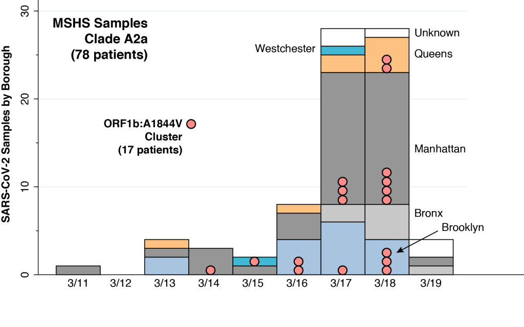
The original article on the MSHS sample did not provide the dates when the individual virus samples were drawn. However, we were able to reconstruct those dates for 78 MSHS patients in the A2a clade by merging one of the virologists’ supplemental data files with a subsequent compilation, as described in the Technical Notes below. The distribution of these patients, according to date of virus sampling and borough of residence, is shown above. In addition to four of the New York City boroughs (Brooklyn, Bronx, Manhattan, and Queens), two of the MSHS A2a patients were from Westchester County (colored cyan) and five patients had unknown residence (colored white).

The MSHS virologists were further able to isolate two genetically homogeneous local transmission clusters within the A2a clade. The larger cluster of these two local transmission clusters consisted of 17 samples sharing a common mutation designated ORF1b: A1844V, as further described in the Technical Notes. These 17 samples are identified in the above graphic as pink bubbles. The earliest sample in this local transmission cluster was drawn from a Manhattan patient on March 14. Another was drawn from a Westchester patient on March 15, and two more from two separate Brooklyn patients on March 16. Within the narrow space of five days, from March 14–18, virus samples with the same signature mutation were found in residents from Brooklyn, Manhattan, Queens, and Westchester County.

The serial interval between the time the infector has COVID-19 symptoms and the time the infectee has symptoms is an estimated 5–6 days. That means the infector (or infectors) of the individuals in the MSHS local transmission cluster were shedding the virus at least during the interval from March 8–13. Given the broad range of the incubation period from infection to symptoms, the infector (or infectors) were in turn infected during the first week in March. That’s when the virus was being propagated throughout the city.

Our analysis should not be construed as implying that just 17 people constituted the nucleus of the New York City pandemic. To the contrary, this sample of individuals provides a window into a large-scale phenomenon that was rapidly occurring throughout the city.

Nor should we attach any biological significance to the particular mutation shared by the 17 individuals in the MSHS local transmission cluster. Just think of the code “ORF1b: A1844V” as nothing more than a shared serial number.

Lest one get the impression that we’ve stretched the data beyond its reasonable limits, we refer to the conclusions of the virologists conducting the MSHS study: “Morever, we found evidence for community transmission of SARS-CoV-2 as suggested by clusters of related viruses found in patients living in different neighborhoods of the city.”

Hypotheses to Knock Down

While there were multiple introductions of SARS-CoV-2 into the city during February and early March, the evidence supports rapid community spread throughout the city during the first week of March. We return to the big-picture question: How did the virus spread so far so fast?

Let’s start with a straw-man: the virus spread through the city’s water supply. After all, that was the big-picture hypothesis that got the Flint, Michigan investigators on the right track. We know that this hypothesis is wrong right off the bat because it is biologically implausible. We know that the virus is air-borne, not water-borne. We know that the virus enters the human respiratory system through the nose and mouth. We don’t get sick drinking the virus.

Here’s another hypothesis to knock down: there was a huge super-spreader sports or entertainment event in late February or early March that fans from all over the city attended. To be sure, March Madness Basketball didn’t start until March 15. But how about the Celine Dion concerts at the Barclays Center on February 28-29 and March 5?

The difficulty with this hypothesis is that there are no reliable, concrete data to support it. Qualified investigators identified super-spreader events arising from a March 10 choir practice in Skagit County, Washington and church attendance during March 6–11 in rural Georgia. A scientific meeting in Massachusetts in late February has likewise been characterized as a super-spreader event. A party in Westport, Connecticut – snarkily dubbed Party Zero – was alleged to be a super-spreader, but formal, reproducible evidence of contagion to New York City has not been forthcoming. In short, no qualified epidemiological investigation has identified a super-spreader event that could have propagated the virus throughout the city in late February or early March.

Transport

Let’s move on to the New City transportation system. We have private transportation, including cars, trucks, private buses, taxis, scooters, motorcycles, app rides, vans, and limousines. And we have public transportation, including buses and subways. Why couldn’t private transportation have served as the super-spreader? Why couldn’t one of the six Brooklyn residents in the MSHS local transmission cluster have commuted by car to his work in Manhattan? Of course, that’s possible. But there’s a problem. The math doesn’t add up.

One of the distinguishing features of New York City, as the Metropolitan Transit Authority (MTA) has noted, is its massive public transportation system.

The MTA network comprises the nation’s largest bus fleet and more subway and commuter rail cars than all other U.S. transit systems combined. It provides over 2.6 billion trips each year, accounting for about one-third of the nation’s mass transit users and two-thirds its commuter rail passengers. … While nearly 85 percent of the nation’s workers drive to their jobs, four-fifths of all rush-hour commuters to New York City’s central business districts use transit, most operated by the MTA, thus reducing automobile congestion and its associated problems.

The MTA Network: Public Transportation for the New York Region

If private cars, vans and trucks were the critical mechanism underlying the rapid geographic dispersion of SARS-CoV-2 in densely populated urban areas, one wonders how New York City alone could have become the singular epicenter of the COVID-19 pandemic in the United States.

That leaves us with the public transportation system, particularly New York City’s public subway system. We continue to stress the word system, because we should think of the subways not as a loose aggregate of individual stations docked in individual neighborhoods, but as a whole, as a mechanism for efficiently pooling millions of individuals into one large mixing basin.

New York City’s unique subway system had the capability in late February and early March to rapidly disperse SARS-CoV-2 throughout the city’s boroughs – faster than a speeding bullet, able to leap under tall buildings in a single bound.

This is the first article in a series about the earliest days of the coronavirus epidemic in New York City.

Technical Notes

To identify the dates of sampling and boroughs of residence of viral samples from the A2a clade in the MSHS study, we merged two databases:

• the tab entitled Clade A2a GISAID IDs within in the spreadsheet Data File S2, posted in the Supplementary Materials of the MSHS article ; and
• a spreadsheet entitled Download Supplementary Table 2 posted in the Supplementary Materials of a later study of COVID-19 patients treated within the New York University Langone Hospital system.

We merged the two files on the unique common identifier variable gisaid_epi_isi. (GISAID stands for Global Initiative on Sharing All Influenza Data.) This gave a total of 78 MSHS viral samples within the A2a clade.

Next, we used the variable strain in the merged file to identify the 17 virus samples specifically highlighted as sharing the ORF1b:A1844V mutation in the New York Cluster 1 in Figure 2C of the main MSHS article. These 17 samples are indicated as the pink bubbles in our figure above.

We reproduce the two MSHS New York clusters from the original Figure 2C here, changing only the color coding to match our own scheme above, and dropping the bootstrap support values indicated in the original figure. The strain descriptors are shown next to each sample. For example, the strain at the very top of the figure (NY-PV08127/2020) was derived from a viral sample drawn on 3/14/2020 from a Manhattan resident. The red lines show the branches of the phylogenetic tree corresponding to the two NY clusters. The lilac lines refer to background branches from a larger worldwide database of samples. The entire tree is part of a larger branch containing the A2a clade.

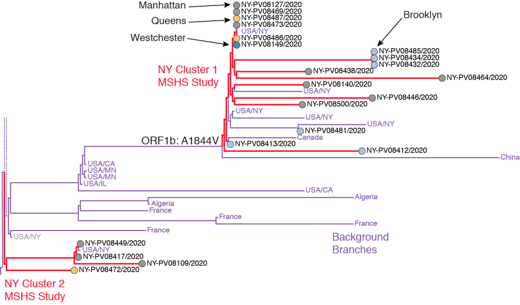
The ORF1b: A1844V mutation shown at the origin of NY Cluster 1 branch refers to a specific base substitution in the stretch of the virus’ RNA that codes for its ORF1b protein, which is one of the two replicase proteins common to SARS coronaviruses. At amino acid position #1844 in this protein, the mutation specific to the MSHS NY Cluster 1 resulted in a change in the resulting amino acid from alanine (A) to valine (V). In terms of the virus’ underlying genetic code, the mutation corresponded to a single base substitution in the virus’ positive-sense mRNA codon from GUX to GCX, where G = guanine, U = uracil, C = cytosine, A = adenine, and X = any of these four bases. This single RNA base substitution (or missense mutation) was shared by samples of infected persons residing in Manhattan, Queens, Brooklyn and Westchester County.