Month: November 2020

Even during the current surge, communities with the highest proportion of multi-generational households have seen the largest increase in new COVID-19 cases. To break the chain, we need to test entire households, and not just individuals.

Four Phases

Figure 1 below shows the weekly incidence of newly diagnosed COVID-19 cases in Los Angeles County, running from the week starting March 1 through the week starting November 8, 2020. When we last studied the Los Angeles County epidemic, we saw three distinct phases. Now, we can clearly see four.

During Phase I, which ran through the week of April 4–10, the epidemic spread radially from initial foci of infection located in relatively affluent communities such as the Brentwood and Beverly Crest neighborhoods of Los Angeles and the City of West Hollywood. During Phase II, which ran through the week of July 5-11, COVID-19 incidence rose at slower rate, as coronavirus infections became increasingly concentrated in areas at higher risk of intra-household transmission. During Phase III, which continued until the week of August 30-September 5, COVID-19 incidence gradually declined, while cases continued to accumulate in the same high-risk areas.

Now, we’re in the midst of Phase IV, and cases are again surging. We’ve cut off our graph at the week of November 8-14, as reporting delays prevent us from accurately gauging the full extent of the recent surge. But the incidence of new cases will undoubtedly continue to rise.

Multi-Generational Households

Figure 2 compares two maps of Los Angeles County. Each map is broken down into countywide statistical areas (CSAs), a hybrid geographic classification of independent municipalities such as the City of Beverly Hills, neighborhoods of Los Angeles such as Hollywood, and unincorporated places such as Hacienda Heights.

On the left, the CSAs are color-coded according to the age-adjusted cumulative incidence of COVID-19 per 100,000 population as of November 26, 2020, which we derived from the surveillance dashboard of the Los Angeles County Department of Public Health. On the right, the same CSAs are coded according to the proportion of households that we’ve identified as at risk for multi-generational transmission, which we derived from the 2018 public use microsample of the U.S. Census Bureau’s American Community Survey. As explained in this detailed report, we classified a household as at risk for multi-generational transmission if it had at least four persons, at least one person 18–34 years of age and another person was at least 50 years of age.

The two maps in Figure 2 show just as striking a concordance as when we last performed the comparison. Those communities with the highest prevalence of at-risk households had the highest cumulative incidence of COVID-19 infection.

Within-Household Transmission Has Sustained the Los Angeles County Epidemic

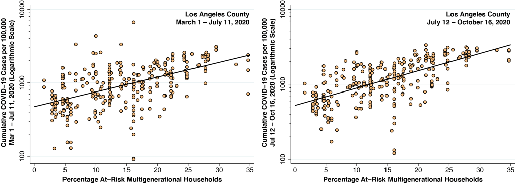
Figure 3 duplicates a pair of graphs that we displayed in our last look at the Los Angeles County epidemic. Both relate the cumulative incidence of COVID-19 infection on the vertical axis to the prevalence of at-risk households across some 300 CSAs in Los Angeles County, as measured on the horizontal axis.

The graph on the left covers cases of COVID-19 diagnosed during Phases I and II, from March 1 through July 11, 2020, when weekly incidence rates were continuing to rise. The graph on the right, by contrast, covers cases diagnosed during Phase III, from July 12 through October 16, when weekly incidence rates turned around and gradually began to fall. Both graphs show a significant positive relationship between the prevalence of at-risk, multi-generational households and the incidence of newly diagnosed coronarvirus infections.

The Catch

Figure 4 repeats the same analysis, covering the cumulative incidence of new cases during Phase IV, from October 17 though November 26. Once again, there is a significant positive relationship across communities between the prevalence of multi-generational households and the incidence of new infections.

The only difference between the plots in Figure 3, which cover Phases I through III of the epidemic, and Figure 4, which covers Phase IV to date, is that the slope of the Phase IV plot is flatter. It remains to be seen whether the slope will stay flatter as backlogged case reports finally make it to the LA County dashboard. If so, it could be an indicator that, while multi-generational household transmission is still a critical vehicle for sustaining the epidemic, the virus has begun to spread outside its established areas of concentration. We need to follow this relationship closely in the coming weeks.

The Negative Feedback Loop

A number of factors, operating in combination, may have triggered the Phase IV surge in Los Angeles County. While it’s nowhere near as cold in Southern California as other parts of the country, nevertheless people are beginning to spend more time indoors. Rising infection rates elsewhere may have led to more importations from outside the county. And then, as we have repeatedly seen in Los Angeles and elsewhere, there is the obvious negative feedback loop. When the epidemic becomes more severe, public officials impose restrictions on social mobility and people take more protective measures. And when the epidemic starts to dissipate, public officials relax restrictions and people drop their guard. That’s why we see the cycles underlying the epidemic curve in Figure 1.

The Multiplier

Whatever the underlying trigger for Phase IV, the high prevalence of multi-generational households in many communities in the Los Angeles area operates as a multiplier. As we noted in our last look, when a younger person, having contracted COVID-19 outside the household, brings his or her infection back home, the impact is magnified by the presence of cohabitants of multiple generations. During our own clinical work, we have recently noted a significant resurgence in the number of infected patients seeking care and advice. Every one of these patients, without exception, has been part of a multi-generational household.

Test Households, Not Just Individuals

A symptomatic patient calls seeking medical advice. She started to feel ill yesterday, but today she has body aches, spiking fevers, and can’t smell her food. She wants to know whether she should get tested. Except as a formality, testing this symptomatic patient is completely uninformative. If the test comes out positive, well, we already knew from the patient’s clinical presentation that she was infected. (A sudden loss of smell in the absence of a completely blocked nose is, by itself, a highly specific test for COVID-19.) And if the test comes out negative, then it was quite likely a false negative and needs repeating.

So, what do we advise the patient? Absolutely everyone in the household has to be tested as soon as possible. Everyone from the toddlers up to the grandparents. The patient may be the first to seek care, but with the high rate of asymptomatic transmission, we need to proactively find out who introduced the infection into the household, who remains susceptible, and who is at risk for the development of severe symptoms in the coming days.

Clusters or networks of places – and not just individual sites – may play a critical super-spreading role.

When we think of super-spreader events, we tend to focus on places with a high concentration of susceptible people, such as assisted living facilities, detention centers, sports arenas, food processing plants, and other mass gatherings at a single site.

To better understand how the coronavirus can spread rapidly, we need to think more broadly about clusters or networks of places, and not just one place at a time. The idea is that infected individuals can move easily and rapidly across multiple places within the cluster or network. The component places are in turn linked together by close geographic proximity, or by an efficient transportation network.

Last spring, to take a salient example, South Korean authorities reported an outbreak of 34 cases after a 29-year-old patient visited five clubs and bars in the Itaewon district of Soeul from the night of May 1 to the early hours of the following morning. Case tracking eventually identified a total of 246 primary and secondary infections.

This super-spreader model underlies our analysis of the possible role of a cluster of off-campus bars in a recent outbreak at the University of Wisconsin-Madison, where nearly three thousand students tested positive for SARS-CoV-2 during September 2020. For a detailed exposition of our data sources, analytical methods and findings, see our National Bureau of Economic Research Working Paper 28132.

Green, Red, Purple and Yellow

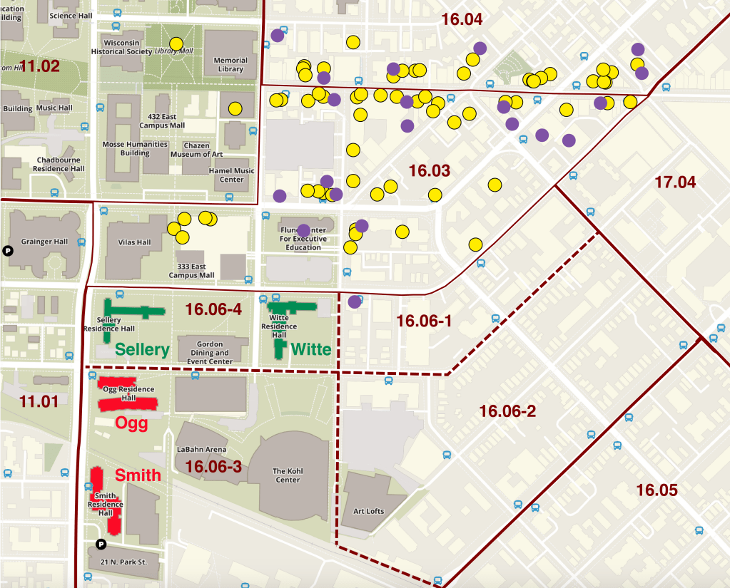
Figure 1 shows a screenshot of a section of the university campus map, focusing on the eastern end of the campus. The superimposed solid lines mark the external boundaries between the census tracts, while the dashed lines mark the internal boundaries between the four census block groups within census tract 16.06.

The pair of green buildings within census block group 16.06-4 represent the two on-campus residence halls, Sellery and Witte, which were subject to a lockdown when approximately 20 percent of their residents became infected.

The pair of red buildings further to the south within census block group 16.06-3 represent two other residence halls, Ogg and Smith, that were not overrun with infections and not subject to quarantine.

The solid purple circles mark the locations of a cluster of 20 nearby off-campus bars, located mostly in census tracts 16.03 and 16.04.

The yellow circles show a comparison group of 68 coffee houses, inexpensive and medium-priced restaurants located in the same area. These venues are closer to Sellery and Witte than to Ogg and Smith. The most remote bar was only a 13-minute walk from Sellery.

Case Control Study

These four graphic elements – the green pair of residence halls , the red pair of residence halls , the purple cluster of bars , and the yellow group of restaurants – form the basic components of a case control study.

In the typical case control study, researchers want to find out whether exposure to a particular toxin is associated with the development of a particular disease. To that end, the researchers identify two categories of individuals. Those who have come down with a disease are the cases , and those who did not get the disease are the controls. The researchers then determine the odds that someone from the cases was exposed to the toxin. Similarly, they determine the odds that someone from the controls was exposed to the toxin. The ratio of these two quantities is called the odds ratio, which is routinely computed in a research report of the study.

For example, in the classic case control study of smoking and lung cancer reported by Richard Doll and Bradford Hill in 1950, the cases were hospitalized patients with lung cancer and the controls were patients without lung cancer. The odds that a patient with lung cancer (one of the cases) was a smoker were 2.97 times the odds that a patient without lung cancer (one of the controls) was a smoker.

In our study, the cases were residents of Sellery and Witte , while the controls were residents of Ogg and Smith . While not everyone in Sellery and White tested positive for COVID-19, it’s enough to know that the rate was much higher Sellery and White than in Ogg and Smith, so much higher that Sellery and White had to be put under quarantine.

In the classic Doll-Hill study, hospitalized patients were interviewed about their smoking habits. In our study, we used anonymized smartphone tracking data from the SafeGraph Patterns database to determine how many devices originating in Sellery-White (census block group 16.06-4) and Ogg-Smith (census block group 16.06-3) visited bars (the purple circles ) or restaurants (the yellow circles ). The odds that a Sellery-White resident (one of the cases) visited a bar were 2.95 times the odds that an Ogg-Smith resident did so. By contrast, the corresponding odds ratio for visiting the restaurants (the yellow circles) was only 1.55.

The SafeGraph data tell us only how many devices originating in a particular census block group visited a particular point of interest (in this study, a bar or a restaurant). The data aren’t broken down by individual smartphone, so we don’t know how many devices visited specific combinations of bars or restaurants. Still, we do know that the odds ratio for visiting a bar was almost twice the odds ratio for visiting a restaurant.

Observational Studies versus Experiments

Our case control study is an observational study. It is not an experiment in which subjects are randomly assigned to visit bars or restaurants to see who comes down with COVID-19. Accordingly, it is at least arguable that people who go to bars are less likely to wear masks, maintain social distancing, and take protective measures generally. The same criticism could be applied to a study of people who attended a political rally, a motorcycle rally, or a large wedding reception. Still, our comparison of residence halls – rather than individuals – tends to blunt this criticism.

There are numerous factors that go into a student’s decision to live in one residence hall versus another – whether the rooms are singles or doubles, whether there is more than one bathroom on a floor, whether the floors are mixed coed, whether the rooms have carpeting or air conditioning, and whether the student can cohabit with his or her friends, not to mention the price. It would be a stretch to argue that these factors readily correlate with a lack of protective behavior.

Party Dorms

One could, of course, speculate about other possible explanatory factors. Sellery and Witte were regarded by some observers as party dorms, at least during prior semesters. This raises the possibility that some smartphone visits to the 20-bar cluster were to purchase alcoholic beverages to bring back to residence hall parties. But that wouldn’t negate the causal role of the bars in facilitating the parties.

Another possible explanation is that residents of Sellery and Witte partied at off-campus fraternities and sororities. But the smartphone tracking data from the SafeGraph Social Distancing database do not show a large number of visits from census block group 16.06-4 (where Sellery and White was located) to census block groups 16.04-1 and 16.04-4 (where the fraternities and sororities were concentrated).

A better explanation is that, with the preventive measures taken by the university, a substantial portion of the alleged partying was shifted off-campus. While some of the partying could have taken place in off-campus private residences, the smartphone tracking data tell us that a significant proportion was shifted to off-campus bars .

Incoming Freshman

Sellery and Witte had more incoming freshman than other residences. To the extent that Wisconsin’s legal age limit of 21 was strictly observed, it would tend to reduce the visitation rate of these residence halls to local bars. Incoming students are required to enroll in an on-campus meal plan, which might help to explain why off-campus restaurant visitation appeared to be a less important predictor of the higher rate of infections at Sellery and Witte. On the other hand, Smith Residence Hall had its own Starbucks, which would tend to reverse that trend.

Proximity

If there is any factor that clearly distinguishes Sellery and Witte from Ogg and Smith, it is that one pair of residence halls is nearer and the other pair is farther away. But that begs the question: Nearer to or farther from what? Our findings fit with the conclusion that the residents of Sellery and White suffered significantly more infections than the residents of Ogg and Smith because they were nearer to the 20-bar cluster, and not because they were also nearer to coffee houses, inexpensive and moderately priced restaurants, or nearer to some classrooms.

The Timing is Right

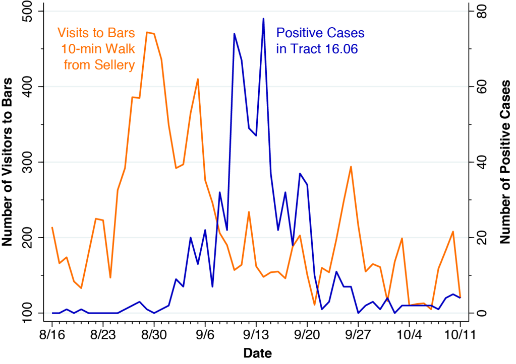
Figure 2 contains two concurrent plots covering each day from August 16 through October 11. The orange line, measured on the left vertical axis, shows the total number of daily visits by all devices, without restriction on origin, to any one of the eleven bars in the cluster within a 10-minute walk of Sellery. Since the SafeGraph Patterns database tracks the GPS pings emitted from a limited panel of devices, only the relative changes in visit counts have significance. Thus, during the week of August 16, there was an average of 176 daily visits among device-holders in the SafeGraph panel to the eleven bars. During August 29-30, the number peaked at 471, a relative increase of 2.7-fold.

The blue line, measured on the right vertical axis in Figure 2, shows the daily number positive COVID-19 cases reported by the Wisconsin Department of Health Services (WDHS) for census tract 16.06. (WDHS reported COVID-19 cases by census tract, but not by census block group.)

Comparison of the orange and blue data series shows a double-peaked surge in the volume of bar attendance, with the first peak occurring on August 29-30 and the second on September 5. Soon thereafter, the double-peaked surge in the volume of bar attendance was followed by a double-peaked surge in positive SARS-CoV-2 cases, with the first peak on September 10 and the second on September 14.

The timing is entirely consistent with a causal relationship between the two trends. The delay between the two curves in Figure 2 represents the latency period between initial infection and the subsequent onset of detectable disease.

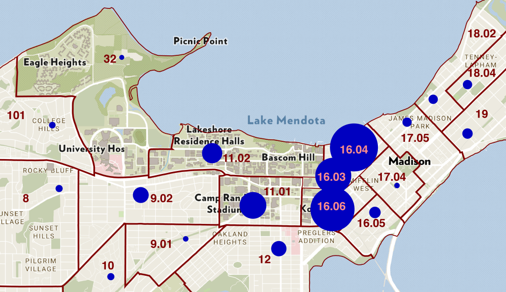
Zooming Out

In Figure 3, we have zoomed all the way out on our campus map. Now we can see the entire campus, along with all the surrounding census tracts. This time, we’ve annotated the campus map with blue bubbles indicating the number of positive COVID-19 cases in each surrounding census tract reported by WDHS during the two-month interval August 16 – October 16. The cumulative number of cases is proportional to the area (not the diameter) of each bubble. The four largest bubbles are: tract 16.04 (870 cases); tract 16.06 (726 cases); tract 16.03 (488 cases); and tract 11.01 (266 cases). These four census tracts comprised 76.7 percent of the 3,065 cases in campus-area census tracts compiled by WDHS during this 2-month interval.

The data in Figure 3 make clear that the cluster of 20 bars – concentrated in tracts 16.03 and 16.04 – was located directly within the geographic epicenter of the outbreak.

Census Tract Study

Figure 3 suggests another way of analyzing the data. Rather than comparing individual residence halls, we could treat individual census tracts as the units of analysis.

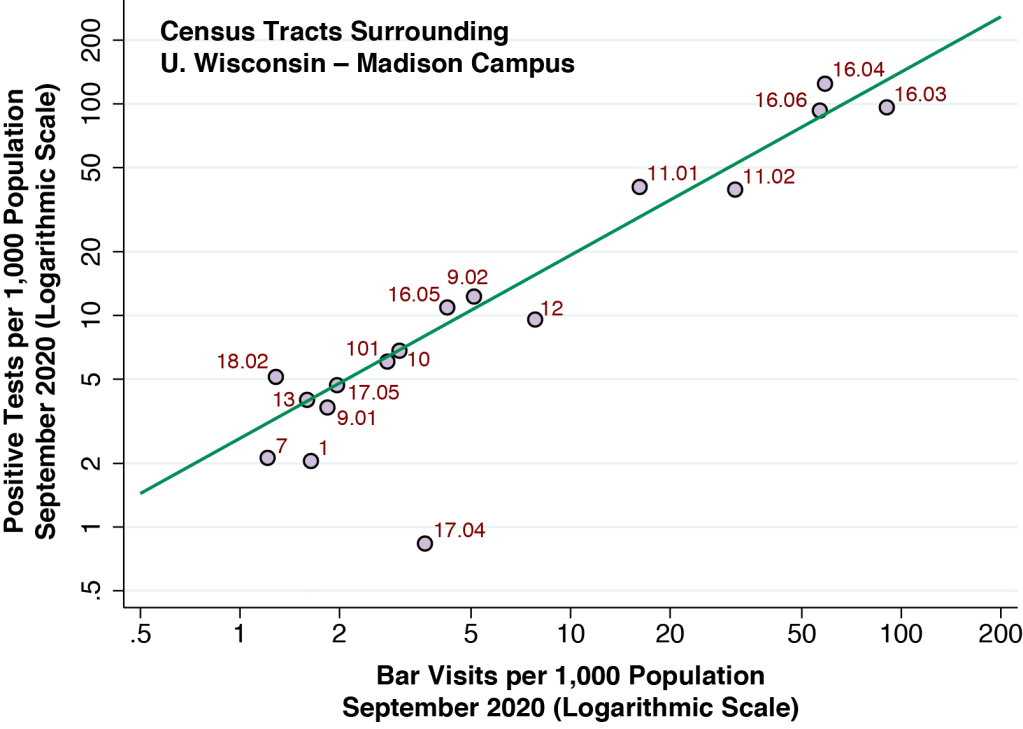
That’s exactly what we’ve done in Figure 4 below. The each lilac-colored point on the graph corresponds to a census tract. The vertical axis measures the number of positive coronavirus tests per 1,000 population in each census tract, while the horizontal axis measures the number of bar visits per 1,000 population by the census tract of origin of the bar visitor. Both axes are on a logarithmic scale so that, for example, the distance between 2 and 10 (that is, a 5-fold increase) is the same as the distance from 10 to 50.

With the exception of one outlier (tract 17.04), the points are aligned along the green fitted line. The slope of the fitted line was 0.87. Economists interpret this slope as an elasticity. For every 10-percent increase in bar visits per capita, the incidence of COVID-19 cases per capita rises an estimated 8.7 percent.

When we constructed the same graph for the per-capita number of visits to the group of 68 restaurants, the data did not fit anywhere near so tightly as in Figure 4. When we performed a multivariate regression, we again found a significant relation to bar visits (with an elasticity of 0.90) and no significant relation to restaurant visits. This finding was entirely consistent with the results of our case control study.

What Have We Learned

In contrast to studies of outbreaks that focus sharply on a single location, our study concentrated on a cluster of places, in this case a cluster of bars right in the geographic epicenter of the outbreak.

While we posited that a cluster or network of places can serve as a super-spreader, we did not have sufficient data in this study to map out the individual connections between places. We had some data on the movements of smartphone holders from one census block group to another, but we would need an even finer geographic grid to ascertain how the connections between bars within a census block group unfold. Still, it would be inappropriate to assume that, in absence of hard data, each establishment in the 20-bar cluster had no more than an independent effect on the risk of coronavirus propagation.

Our findings should not be interpreted broadly to mean that restaurants are entirely free of risk while bars are the sole source of contagion. The narrower interpretation is that a specific, centrally located cluster of bars appeared to be a significantly greater vehicle for propagation of the virus than restaurants in a particular university-based outbreak. Neither do our findings point the finger at all bars. Among the 51 bars throughout the campus area, we focused sharply on a cluster of 20 bars at the geographic epicenter of the outbreak.

Perspectives

Future studies of college and university outbreaks need to concentrate harder on the dynamics of viral transmission, and not simply on how many cases ended up in dormitories, athletic teams, fraternities and sororities. Retrospective case-tracking needs to expand its scope to ask an infected individual not just whether he went to a bar, but also whether he went bar-hopping, whether his roommates also went to bars, and if so, to what bars on what nights.

We need to think more about the ways that multiple places within a cluster may act synergistically to enhance viral propagation. The outbreak in the Itaewon district of Soeul, cited above, points to a model where an index case moves from one place to another within the cluster. More generally, when there is high mobility between places, they may function effectively as one place. If an average of 20 patrons attended each of five interconnected bars on a single night, we would end up with an “event” with 100 attendees. When a student says to his friends, “Let’s go to bar A and if we can’t get in, we’ll just go to bar B,” we have a classic network externality where the mere availability of bar B enhances the demand for, and thus the transmission potential of, bar A.

Even more broadly, we need to think about systemic factors that influence viral propagation, and not simply the characteristics of individuals or the places they go to. The epidemic in Los Angeles County has been sustained in great part by intra-household transmission among multigenerational families. But the larger question is what public policies have enhanced or mitigated these housing conditions. The spread of coronavirus in New York City and other metropolises may have been enhanced by individuals of high mobility. But the larger question is what transportation networks carried them from one place to another.